Time Series

Analyze time-based data and forecast future behavior

Time Series is a representation of numeric data that is indexed sequentially over equally distributed data points in time. Annual grain production expressed in tons, pressure sensor readings that are produced every minute or the daily closing value of the Dow Jones Industrial Average are some examples of such temporally ordered data. Time Series are generally used to analyze time-based data to extract meaningful statistics and other characteristics of the data or when historical patterns can explain the future behavior. Time Series forecasting involves training a model on historical data that can be used to make forecasts for the future values of chosen numeric fields.

Sign up now! It's free!

Applications of Time Series

Serialized time-based data expressing historical patterns are widely available in many industries. As a result, the application areas for Time Series are equally diverse. In addition to sales, demand and weather forecasting, predicting stock prices, website traffic, production and inventory levels, and macroeconomic metrics represent only a small subset of use cases, where Time Series can be utilized.

Best-in-class algorithm

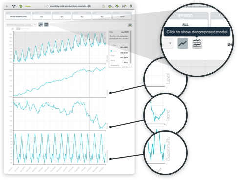
You can create time series with a dataset containing one or more numeric fields with time series data. By Default, BigML Time Series replace missing values using spline interpolation. Under the hood, BigML Time Series implements exponential smoothing methods. The smoothing parameters assign exponentially increasing weights to more recent instances. Time series data is modeled as a level component and it can optionally include a trend (damped or not damped) and a seasonality components. Both trend and seasonality components have two variations: additive or multiplicative. The additive variation of trend uses Holt's linear method as the trend growth is assumed to be linear whereas the forecast equation with multiplicative trend uses exponential trend method, i.e., it contains is a constant growth rate that is multiplied by the level component. Because most real world trend models aren't repeated indefinitely you can "dampen" the trend to a flat line if forecasting a long time horizon. Together, the trend, the seasonality and the error components and their variations yield up to 19 automatically generated models as you create a BigML Time Series, which results in significant time savings.

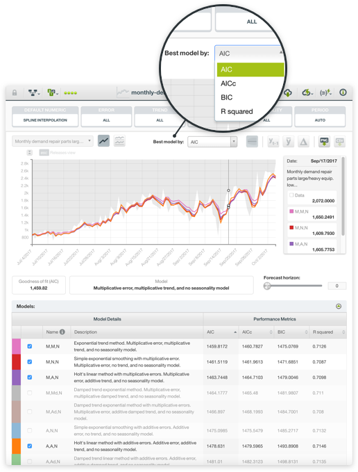
Each model learned from the training data, BigML provides a set of performance metrics: AIC (Akaike's Information Criterion) measures the trade-off between the goodness-of-fit and the model's complexity; AICc (Corrected Akaike's Information Criterion) introduces a correction element that is useful for smaller datasets; BIC (Schwarz Bayesian Information Criterion) is akin to AIC, but it penalizes the model's complexity more heavily; and finally, R squared measures the model's errors compared to the objective fields' actual values that mimic a benchmark model that always predicts the mean.

Highly interpretable results

When your Time Series has been created, you get a chart that shows the original training data for each objective field along with the data points go for the best performing model by the AIC metric, which is the default. In addition to the "Goodness of fit" value, the chart also includes the estimates for up to next 50 data points for each fitted model. However, BigML fits up to 19 different models that are automatically learned from your training data and they are all displayed with accompanying performance metrics in case you'd like to apply a different ranking. These competing models are varied by different combinations of the forecast components (error, trend, seasonality) and their configurations (multiplicative, additive, damped, not damped).

Time Series evaluations

Time Series evaluations let you measure the performance of Time Series models, if you have already set aside some testing data by applying a linear split to your dataset. The evaluation chart shows the selected model forecasts for the testing data, which allows you to visually analyze the goodness-of-fit of all the underlying Time Series models. By default, BigML selects the model with the best R squared metric, but you can select the best model by other evaluation metrics such as the MAE, MSE, sMAPE, or MASE. The forecast data points for the test data are plotted along with a confidence interval. This is the error interval in which the forecast is expected to be located with a confidence of 95%.

Real-time or customizable Topic Distributions

Once you create a Time Series model, you can make Forecasts to predict the future values of your chosen target numeric fields. BigML requires a time horizon to compute Forecasts, and you can optionally include a confidence interval to your Forecasts.

Fully programmable Time Series

In addition to the point-and-click mode on BigML Dashboard, you can programmatically create, list, delete, and use your Time Series or your Time Series evaluations through the BigML's REST API and bindings for all popular languages. You can choose to use BigML with Python, Node.js, Java, Swift, C# or other languages. Time Series are also supported by WhizzML, our domain-specific language for automating Machine Learning workflows, implementing high-level Machine Learning algorithms, and sharing them with others.

Time Series Training Video